Trading Root Lookup Traffic for Replicated State in a Tree Network
1. The Design Question
A tree-structured naming system can resolve an identifier through a root directory or through a server whose address the client already knows. Two designs may require the same number of lookup steps while placing very different loads on the root.
This post compares two ways to distribute address information. In the first, every node stores address records for all its descendants. In the second, the root stores the global directory, while non-root nodes store only their direct children’s addresses.
The question is how much root lookup traffic the additional replication can save, and what it costs to keep those replicas up to date. I use a simplified tree and cache model to examine this trade-off.
2. Two Ways to Store Address Information
Consider a perfect $x$-ary tree of depth $h$, with the root at depth $0$. Each node is a server identified by a hierarchical name, such as a.b.c.
The client always knows the root’s address and may cache the addresses of other nodes after successful lookups. We consider only requests for targets whose addresses are not already cached.
2.1 Scheme 1: Subtree Replication
In Scheme 1, each node stores address records for all nodes in its subtree. As a result, any cached ancestor of a target can resolve that target directly.
If the client has cached multiple ancestors, it uses the deepest one as the lookup entry point. If no non-root ancestor is available in the cache, the client queries the root.
2.2 Scheme 2: Global Directory with Local Child Records
In Scheme 2, the root stores address records for all nodes, while each non-root node stores records only for its direct children.
The client can bypass the root only when the target’s direct parent is already cached. Otherwise, it sends the lookup request to the root.
For example, suppose the client wants to resolve a.b.c.d.
If a.b is cached, Scheme 1 can use it to resolve the target because a.b is an ancestor of a.b.c.d. Under Scheme 2, node a.b stores records only for its direct children, so it cannot resolve a.b.c.d. It must therefore fall back to the root.
If a.b.c is cached, both schemes can use it because a.b.c is the target’s direct parent.
3. Modeling Root Lookup Traffic
3.1 Tree Size
The total number of nodes in the tree is $$ N = \sum_{i=0}^{h} x^i = \frac{x^{h+1}-1}{x-1}. $$
of these nodes, $x^h$ are leaves and
$$ I = N - x^h = \frac{x^h-1}{x-1} $$
are internal nodes. For large $h$,
$$ \frac{I}{N} \approx \frac{1}{x}. $$
Thus, a uniformly sampled node is much more likely to be a leaf than an internal node. This fact will help explain why caching $t$ nodes dose not generally provide coverage for $tx$ targets under Scheme 2.
3.2 Cache Model
We firstwanalyze a single client. Let $S$ denote the set of non-root nodes whose addresses the client has cached, and let $$ |S| = t. $$
3.3 Scope and Assumptions
先分析单个客户端。
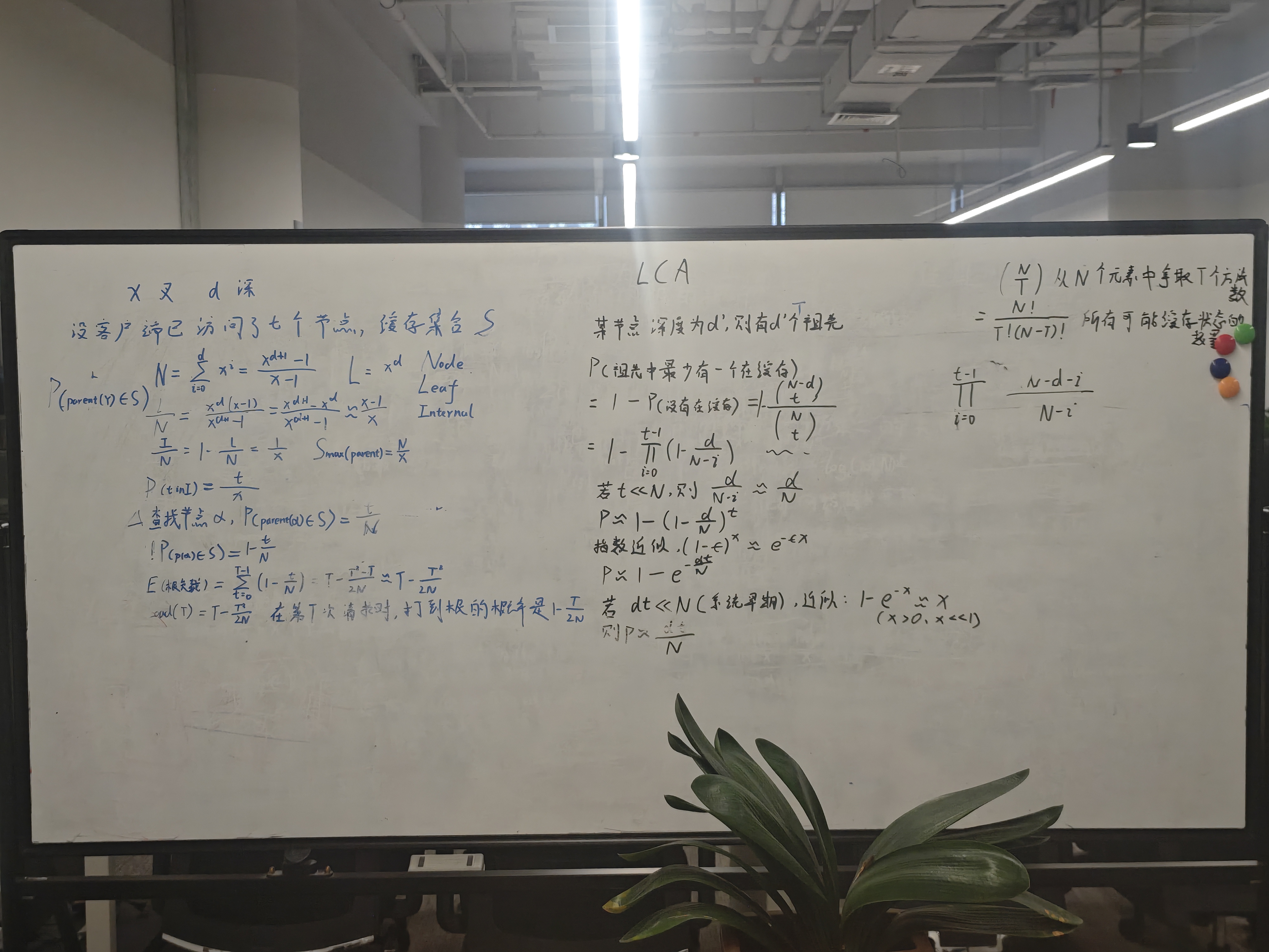
设客户端已经缓存了 (t) 个不同节点,缓存集合记为:
$$ S $$
其中:
$$ |S| = t $$
先采用一个简化模型:这 (t) 个缓存节点可以近似看作从全网 (N) 个节点中均匀随机抽出的 (t) 个节点。
因此,对于任意一个固定节点 (u),它在缓存中的概率是:
$$ P(u \in S) = \frac{t}{N} $$
这个结论非常重要。
它不是因为 (u) 是内部节点或叶子节点,而是因为缓存是从全部 (N) 个节点中抽取的。对任何一个固定节点来说,被抽中的概率都是:
$$ \frac{\text{缓存大小}}{\text{总节点数}} = \frac{t}{N} $$
4. The Cost of Keeping State Fresh
方案二中,目标节点 (v) 可以绕过根,当且仅当:
$$ parent(v) \in S $$
也就是说,客户端已经知道目标节点的直接父节点。
对于一个随机目标节点 (v),它的父节点是某个固定内部节点。由于任意固定节点在缓存中的概率都是 (t/N),所以:
$$ P(parent(v) \in S) = \frac{t}{N} $$
因此,方案二的免根概率是:
$$ P_{\text{hit}}^{(2)}(t) = \frac{t}{N} $$
根节点被访问的概率是:
$$ P_{\text{root}}^{(2)}(t) = 1 - \frac{t}{N} $$
这就是白板左侧的核心公式。
4.1 为什么不是 (\frac{tx}{N})?
直觉上,已知 (t) 个节点,每个节点最多有 (x) 个孩子,所以似乎最多有 (tx) 个节点可以绕过根。
这个上界没错,但它不是期望值。
原因是:缓存中的大多数节点是叶子,叶子没有孩子。
缓存中内部节点的期望数量是:
$$ t \cdot \frac{I}{N} \approx t \cdot \frac{1}{x}
\frac{t}{x} $$
每个内部节点有 (x) 个孩子,所以它们合计覆盖的孩子数量期望是:
$$ \frac{t}{x} \cdot x = t $$
所以真正的免根候选数量期望是 (t),不是 (tx)。
因此:
$$ P_{\text{hit}}^{(2)}(t) \approx \frac{t}{N} $$
这里的 (x) 被内部节点比例 (1/x) 抵消了。
4.2 方案二的累计根负载
如果近似认为每次请求都会带来一个新的缓存节点,那么第 (s) 次请求前,缓存大小约为 (s)。
第 (s) 次请求访问根的概率是:
$$ 1 - \frac{s}{N} $$
那么前 (T) 次请求的累计根访问次数期望为:
$$ R_2(T) = \sum_{s=0}^{T-1} \left( 1-\frac{s}{N} \right) $$
拆开:
$$ R_2(T) = \sum_{s=0}^{T-1}1
\frac{1}{N} \sum_{s=0}^{T-1}s $$
第一项:
$$ \sum_{s=0}^{T-1}1 = T $$
第二项:
$$ \sum_{s=0}^{T-1}s = \frac{T(T-1)}{2} $$
所以:
$$ R_2(T) = T
\frac{T(T-1)}{2N} $$
当 (T) 较大时,可以近似写成:
$$ R_2(T) \approx T
\frac{T^2}{2N} $$
平均根负载比例为:
$$ \frac{R_2(T)}{T}
1
\frac{T-1}{2N} \approx 1-\frac{T}{2N} $$
注意,这个比例是“累计平均比例”,不是瞬时概率。
瞬时根访问概率是:
$$ P_{\text{root}}^{(2)}(T) = 1-\frac{T}{N} $$
5. What the Model Does and Does Not Tell us
方案一中,每个节点知道自己整个子树内的所有地址。
因此,如果客户端缓存中有目标节点 (v) 的某个祖先节点,那么客户端可以问这个祖先节点,由它直接返回目标地址。
所以方案一绕过根的条件是:
$$ S \cap Ancestor(v) \neq \varnothing $$
其中 (Ancestor(v)) 表示目标节点 (v) 的可用祖先集合。
如果目标节点深度为 (d),那么它路径上的祖先数量与 (d) 成正比。为了避免根节点本身带来的歧义,我们定义:
$$ \ell(v) = \text{目标节点路径上可用于绕过根的缓存前缀数量} $$
在白板推导里,可以近似把:
$$ \ell(v) \approx d $$
理解为:深度越深,路径上可能命中的前缀节点越多。
5.1 固定目标节点的精确命中概率
固定一个目标节点 (v),假设它有 (\ell) 个可用祖先节点。
缓存大小为 (t)。
我们要求:
$$ P(\text{缓存中至少有一个祖先}) $$
用补集更简单。
“至少有一个祖先在缓存中”的反面是:
$$ \text{没有任何祖先在缓存中} $$
总缓存选法数是:
$$ \binom{N}{t} $$
如果缓存中不能包含这 (\ell) 个祖先,那么只能从剩下的 (N-\ell) 个节点中选 (t) 个:
$$ \binom{N-\ell}{t} $$
所以:
$$ P(\text{没有祖先})
\frac{ \binom{N-\ell}{t} }{ \binom{N}{t} } $$
因此:
$$ P_{\text{hit}}^{(1)}(v)
1
\frac{ \binom{N-\ell}{t} }{ \binom{N}{t} } $$
这是方案一对固定目标节点的精确表达式。
5.2 近似成指数形式
当 (N) 很大,且 (t) 相比 (N) 不太大时,可以近似为:
$$ \frac{ \binom{N-\ell}{t} }{ \binom{N}{t} } \approx \left( 1-\frac{\ell}{N} \right)^t $$
所以:
$$ P_{\text{hit}}^{(1)}(v) \approx 1
\left( 1-\frac{\ell}{N} \right)^t $$
继续使用指数近似:
$$ \left(1-\frac{\ell}{N}\right)^t \approx e^{-\ell t/N} $$
于是:
$$ P_{\text{hit}}^{(1)}(v) \approx 1-e^{-\ell t/N} $$
当 (\ell t/N \ll 1) 时,再用一阶近似:
$$ e^{-\ell t/N} \approx 1-\frac{\ell t}{N} $$
所以:
$$ P_{\text{hit}}^{(1)}(v) \approx \frac{\ell t}{N} $$
这就是白板右侧的核心近似:
$$ P_{\text{hit}}^{(1)} \approx \frac{d t}{N} $$
它的含义是:
方案一中,一个缓存节点不只覆盖自己的直接孩子,而是可能通过祖先路径覆盖更深的子树。因此命中概率比方案二多了一个“路径长度因子”。
6. Takeaways
不同目标节点的深度不同,所以 (\ell(v)) 不同。
深度为 (k) 的节点数量是:
$$ x^k $$
因此随机访问一个节点时,目标深度的平均值是:
$$ \mathbb{E}[d]
\frac{ \sum_{k=0}^{h} kx^k }{ \sum_{k=0}^{h} x^k } $$
也就是:
$$ \mathbb{E}[d]
\frac{ \sum_{k=0}^{h} kx^k }{N} $$
当 (h) 较大时,由于树的底层节点最多,平均深度接近叶子深度:
$$ \mathbb{E}[d] \approx h - \frac{1}{x-1} $$
所以粗略地可以写成:
$$ \mathbb{E}[d] \sim h $$
而:
$$ h \sim \log_x N $$
因此方案一相比方案二,多了一个大约为:
$$ \log_x N $$
的缓存命中加速因子。
7. 两种方案的根负载曲线比较
7.1 方案二
方案二只利用父节点缓存。
瞬时根访问概率:
$$ P_{\text{root}}^{(2)}(t) = 1-\frac{t}{N} $$
累计根负载:
$$ R_2(T) = T
\frac{T(T-1)}{2N} $$
早期近似:
$$ R_2(T) \approx T-\frac{T^2}{2N} $$
7.2 方案一
方案一利用祖先 / LCA 前缀缓存。
对固定深度为 (d) 的目标:
$$ P_{\text{root}}^{(1)}(d,t) \approx e^{-dt/N} $$
对所有节点平均:
$$ P_{\text{root}}^{(1)}(t) \approx \mathbb{E}_{d} \left[ e^{-dt/N} \right] $$
在粗略近似下,用平均深度代替 (d):
$$ P_{\text{root}}^{(1)}(t) \approx e^{-\mathbb{E}[d]t/N} $$
由于:
$$ \mathbb{E}[d] \sim \log_x N $$
所以:
$$ P_{\text{root}}^{(1)}(t) \approx e^{-t\log_x N/N} $$
8. 核心对比
方案二:
$$ P_{\text{root}}^{(2)}(t) \approx e^{-t/N} $$
方案一:
$$ P_{\text{root}}^{(1)}(t) \approx e^{-t\log_x N/N} $$
所以方案一的根负载下降速度大约比方案二快:
$$ \log_x N $$
倍。
换句话说:
- 方案二需要缓存规模达到 (O(N)),根负载才会显著下降;
- 方案一大约只需要缓存规模达到:
$$ O\left(\frac{N}{\log_x N}\right) $$
根负载就会明显下降。
这就是方案一的数学优势。
9. 但是方案一的存储成本更高
方案一中,每个节点保存自己整个子树的信息。
一个节点的地址会被它所有祖先保存一次。因此总存储量等价于:
$$ \sum_{\text{所有节点 } v} depth(v) $$
也就是:
$$ \sum_{k=0}^{h} kx^k $$
因此:
$$ Storage_1 = O(Nh) $$
因为:
$$ h = \log_x N $$
所以:
$$ Storage_1 = O(N\log_x N) $$
方案二中:
- 根保存全局 (N) 个地址;
- 每个非根内部节点只保存直接孩子;
- 总体仍是线性级别。
因此:
$$ Storage_2 = O(N) $$
10. Read-Write Trade-off
10. 总请求数是否相同?
如果目标节点尚未被客户端直接缓存,那么两种方案都可以做到:
$$ \text{解析入口} \rightarrow \text{目标节点} $$
也就是常数级解析。
所以从“总请求跳数”看,两者差异不大。
真正的区别在于:
$$ \textbf{解析请求打到哪里} $$
方案二中,大量解析请求早期会集中到根。
方案一中,解析请求会更快被分散到树中的各级祖先节点。
因此:
| 指标 | 方案一:LCA / 子树递推 | 方案二:父节点 / 根注册 |
|---|---|---|
| 单次定位跳数 | 常数级 | 常数级 |
| 根负载下降速度 | 快,约 (e^{-t\log_x N/N}) | 慢,约 (e^{-t/N}) |
| 收敛缓存规模 | (O(N/\log_x N)) | (O(N)) |
| 存储开销 | (O(N\log_x N)) | (O(N)) |
| 本质 | 用存储换根负载分散 | 用根中心化换低存储 |
11. 结论
方案一和方案二的核心差异不是“能不能一跳定位”。在你的设定下,两者都可以做到常数级定位。
真正差异是:
$$ \textbf{缓存命中可以覆盖多少潜在目标} $$
方案二中,一个缓存节点主要帮助它的直接孩子,因此命中增长速度是:
$$ \frac{t}{N} $$
方案一中,一个缓存节点如果是目标路径上的祖先,就可以帮助整个子树,因此命中增长速度带有路径长度因子:
$$ \frac{dt}{N} $$
对整棵树平均后,这个因子约为:
$$ \log_x N $$
所以方案一用更高的状态复制成本,换来了更快的根负载下降。
最终可以概括为:
$$ \boxed{ \text{方案一:空间换根负载} } $$
$$ \boxed{ \text{方案二:低存储但根负载收敛慢} } $$
后续如果加入非均匀访问,方案二会因为热点父节点更快进入缓存而改善;如果加入节点信息变更噪声,方案一会因为上推状态更多而面临更高的失效传播成本。这两个因素会改变最终的工程取舍。